Technology
Precompute the reusable subsystem.Keep the host solver in control.
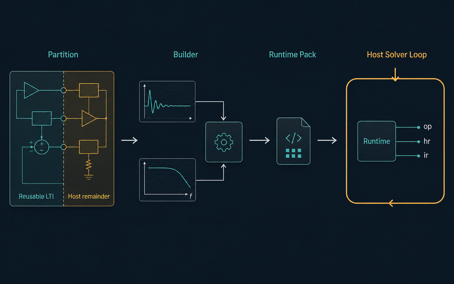
TDSE converts a reusable linear time-invariant subsystem into runtime operator terms, then lets the host solver integrate those terms inside its own time-stepping loop. The host still owns the trial solve, commit sequence, lifecycle policy, and shutdown behavior. TDSE supplies operator data and step-loop terms; it does not take over the host integrator.
↻Repeated computation
Per-step cost: O(N³)
vs
→Reusable operator
Per-step cost: O(P²·L)
Conventional host loop
When the host keeps reopening the same linear subsystem every accepted step, repeated factorization or solve work can dominate runtime. The exact cost depends on solver structure, sparsity, and coupling, but the reusable part is still being revisited inside the live step loop.
TDSE-enabled host loop
TDSE moves that reusable subsystem behavior into precomputed response data and runtime operator terms. At each step, the host queries `op`, `hr`, and `ir`, solves its own equations as usual, and commits the accepted state without reopening the reusable subsystem.
01
Define the reusable boundary
Decide which portion of the coupled model is linear, time-invariant, and worth reusing across accepted steps. This partition is a modeling decision made upstream of the SDK; TDSE assumes that boundary is already defined when response data enters the toolchain.
02
Characterize H and IR
Generate the independent-response and impulse-response content that describes the reusable subsystem at its interface ports. Builder accepts time-domain or frequency-domain response inputs, and Adapter Circuit can supply that data directly for supported circuit-domain workflows.
03
Write the runtime pack
Builder turns those response artifacts into a causal runtime representation and writes a pack file. The pack preserves the operator content, response-history support, and metadata the Runtime layer needs at create time.
04
Integrate inside the host loop
Runtime exposes the step-loop terms `op`, `hr`, and `ir`. The host still owns time stepping, trial versus commit sequencing, and shutdown policy. TDSE contributes reusable operator terms; it does not replace the host solver.
Equation Form
Solver-compatible equation form, expressed as three runtime terms.
At runtime the host does not re-open the reusable linear subsystem. Instead it evaluates an equivalent relation built from an independent-response term, a retained-history term, and an instantaneous coupling term. Those are the pieces surfaced by the Runtime API and consumed by the host step loop.
x[n] =x₀[n]+Σ h[n-k] · p(y[k])+h[0] · p(y[n])
x₀[n]Independent-response term
Precomputed free-response content carried into the current accepted step.
Σ h[n-k] · p(y[k])History-response term
Convolution over retained port history accumulated from previously committed steps.
h[0] · p(y[n])Direct-response term
Instantaneous coupling term aligned with the host solver's current trial state.
In simplified form, the reusable-subsystem contribution scales like
O(Np²·Nh)
Interface count (Np)
Np is the number of exchanged port or interface variables. Runtime work grows with interface dimension rather than with the full internal size of the reusable linear subsystem.
Response history (Nh)
Nh is the retained response-history length. Truncation, history retention, and host integration policy directly affect convolution workload and therefore the amount of reusable-subsystem work performed each step.
Host integration still matters
The scaling expression describes the reusable-subsystem portion of the step loop, not the entire simulation stack. Realized gains still depend on the host solver, memory traffic, scheduling, backend selection, and how the integration boundary is chosen.
Response Sources
Multiple input paths, one runtime shape.
Builder can start from time-domain or frequency-domain response data and normalize it into the same runtime operator form. For supported circuit workflows, Adapter Circuit can provide that response content directly from imported netlists or RAW-based inputs.
Causality
Causality has to be restored before runtime.
Frequency-domain characterization can produce response sequences that look acceptable offline but misbehave inside a live integrator. TDSE applies causality-aware reconstruction and correction before the pack reaches Runtime, so the host consumes a runtime-ready operator rather than raw sampled data.
Host Compatibility
Variable-step hosts still need disciplined integration.
Runtime can serve fixed-step and variable-step hosts, but the host still owns trial, commit, and lifecycle sequencing. The practical requirement is not just mathematical correctness; it is that the operator terms remain well-behaved inside the host's accepted integration pattern and step-size policy.